5. 1D Mode

The 1D / XY mode is the default mode of batplot. It is optimized for XRD but support any generic two-column data. By default, batplot uses the first and second column to plot as x and y, this can be changed using --readcol flag.

Demo XRD wavelengths

In the tutorial / test files:

• TD_R* (e.g. TD_R02.dat) — synchrotron XRD, λ = 0.259 Å
• TD_S0062-64.xy — Cu lab source, λ = 1.54 Å

Plot Any Two-column Data

batplot data.txt --i

plots the first two columns as x and y

Plot XRD Data with Wavelength Conversion

batplot TD_S0062-64.xy --xaxis 2theta --i

plots Cu XRD in 2θ space

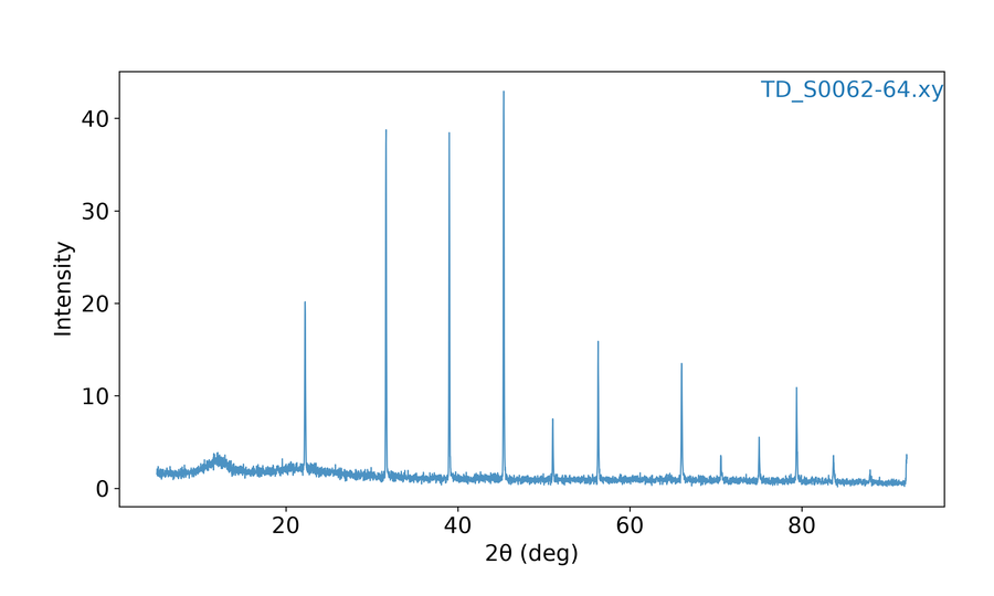
Figure: 2θ (TD_S0062-64.xy, Cu λ = 1.54 Å)

batplot converted/R02.qye --xaxis q --i

plots data already in Q space

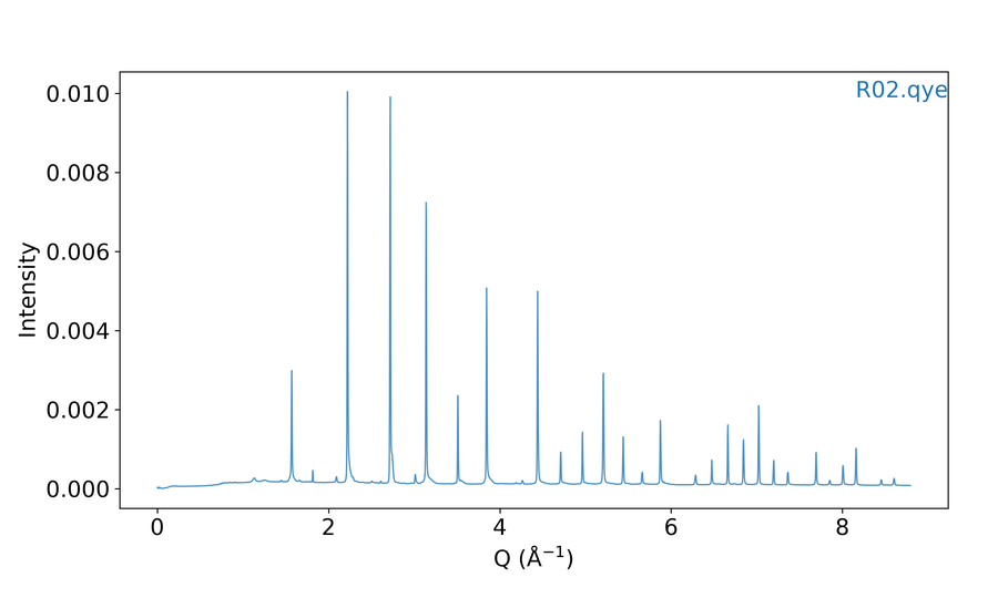
Figure: Q-space `.qye` (converted/R02.qye)

batplot TD_S0062-64.xy --wl 1.54 --i

converts Cu 2θ → Q and plots in Q space

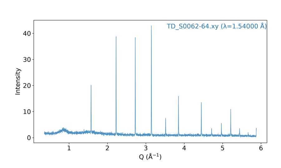
Figure: 1D Q-space (TD_S0062-64.xy, --wl 1.54)

batplot TD_S0062-64.xy:1.54 --i

same conversion using the per-file :λ suffix

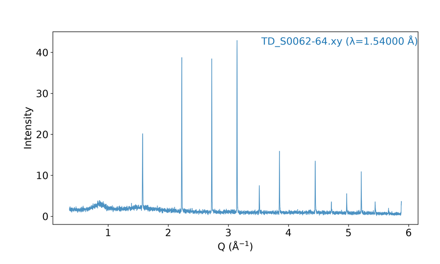
Figure: `:λ` suffix → Q (TD_S0062-64.xy:1.54)

batplot TD_R02.dat TD_R03.dat --wl 0.259 --i

multi-file overlay with the same synchrotron wavelength

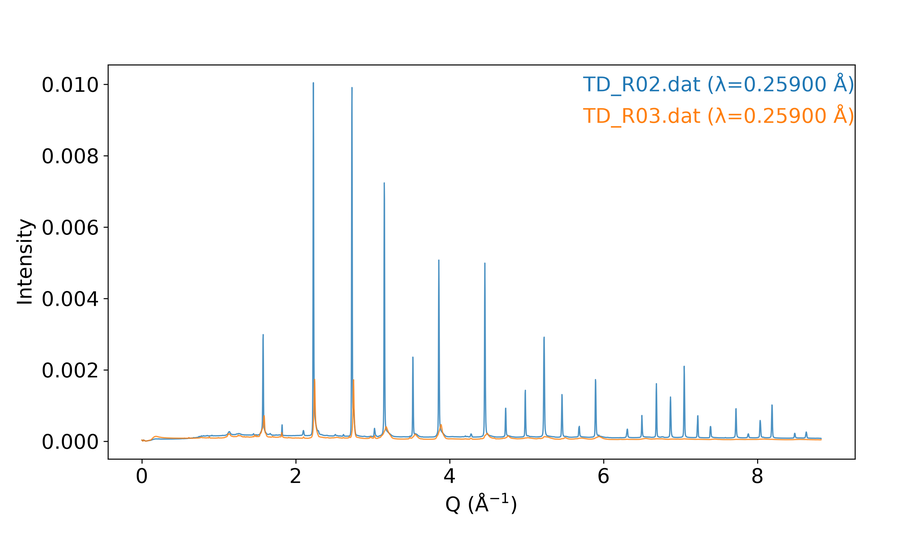
Figure: synchrotron overlay (TD_R02 + TD_R03, --wl 0.259)

batplot TD_S0062-64.xy:1.54 TD_R02.dat:0.259 --i

multi-file overlay with different wavelengths (both plotted in Q)

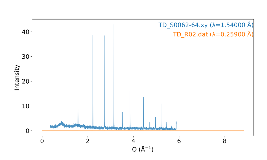
Figure: mixed λ overlay (Cu 1.54 + synchrotron 0.259)

batplot TD_R02.dat:0.259:1.54 --xaxis 2theta --i

re-project synchrotron data into a Cu 2θ frame

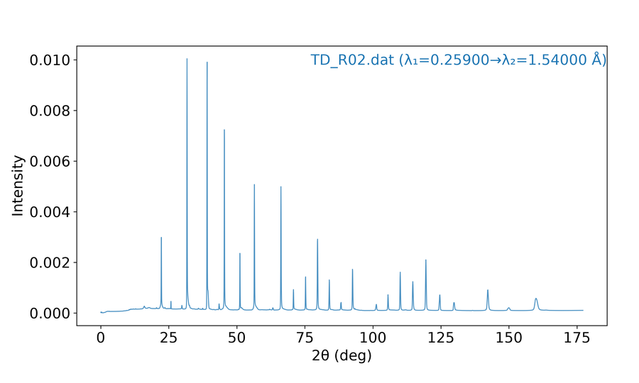
Figure: re-projected 2θ (TD_R02.dat:0.259:1.54)

batplot TD_R02.dat TD_R03.dat --norm --wl 0.259 --i

plots normalized intensity (0–1 scale)

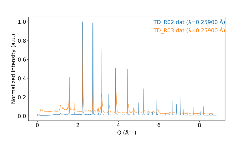
Figure: normalized overlay (--norm --wl 0.259)

Wavelength Handling

batplot converts powder-diffraction X columns among 2θ (deg), Q (Å⁻¹), and (for file export) d (Å). Q and q are always equivalent (case-insensitive).

Plot-time vs file export

Goal	How	Writes new data files?
View 2θ data in Q (or re-project λ) on screen	--wl, file:λ, file:λ1:λ2, interactive u	No — only the figure changes
Save converted columns for other software	--convert	Yes → converted/ next to each input

Relations used

• Q from 2θ: Q = (4π / λ) · sin(θ) with λ in Å and θ = half of 2θ
• d from Q: d = 2π / Q
• 2θ(λ₁) → 2θ(λ₂): convert via Q using each wavelength

Typical λ in the demo set: Cu lab 1.54 Å, synchrotron TD_R* 0.259 Å.

Syntax at plot time

When --wl or a :wavelength suffix is provided, the x-axis becomes Q-space — you do not need --xaxis q (unless you force --xaxis 2theta for a re-projection).

Syntax	What it does
--wl 1.54	Apply one wavelength to all listed data files: convert 2θ → Q.
file.xye:1.54	Per-file wavelength: convert this file’s 2θ → Q (other files can use other λ or none).
file.xye:0.259:1.54	Dual wavelength: treat the file as 2θ at λ₁, re-project to the λ₂ frame (via Q).
file:q	Mark the file as already in Q (no conversion).
phase.cif:1.54	Calculate CIF reference-tick positions in 2θ using that λ.

Examples (terminal style)

batplot TD_S0062-64.xy --wl 1.54 --i

Cu file uses λ = 1.54 Å → plot in Q (figure above)

batplot TD_S0062-64.xy:1.54 TD_R02.dat:0.259 --i

each file keeps its own measurement wavelength (figure above)

batplot TD_R02.dat:0.259:1.54 --xaxis 2theta --i

re-project from synchrotron λ to a Cu-like 2θ frame (figure above)

batplot TD_S0062-64.xy Li2FeSeO.cif:1.54 --xaxis 2theta --wl 1.54 --i

CIF ticks calculated for 2θ at 1.54 Å

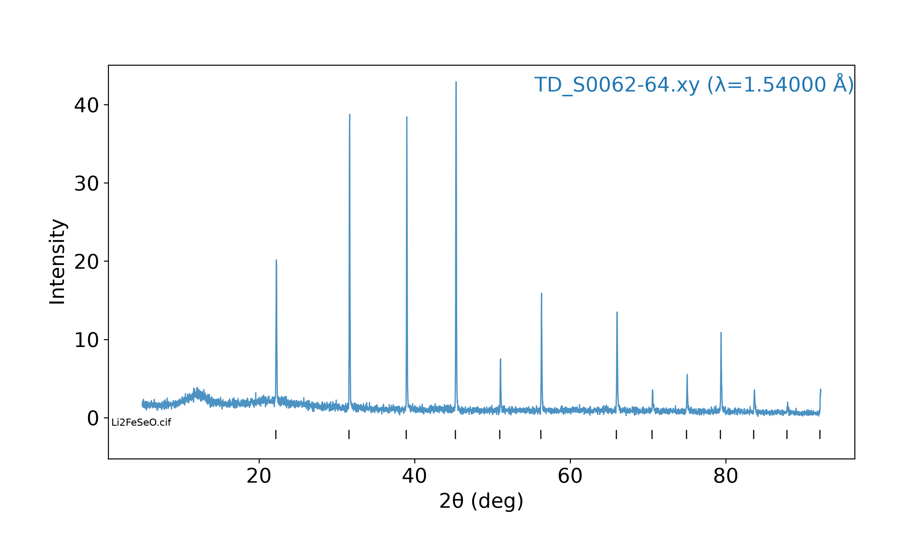
Figure: CIF in 2θ (TD_S0062-64 + Li2FeSeO.cif:1.54)

Note

Any file:wl or file:q suffix implies Q mode automatically (unless --xaxis 2theta wins). Files without wavelength info are then assumed to be already in Q.

Live axis switch inside --i: press u (2θ ↔ Q). To export converted data files, see Convert and export XRD files below and the full --convert chapter.

Using --readcol to Specify Columns

By default batplot plots columns 1 and 2. Use --readcol when you need other columns. Synchrotron file TD_R02.dat has three columns (x, y₁, y₂):

batplot TD_R02.dat --readcol 1 3 --xaxis q --i

plots column 1 as x and column 3 as y

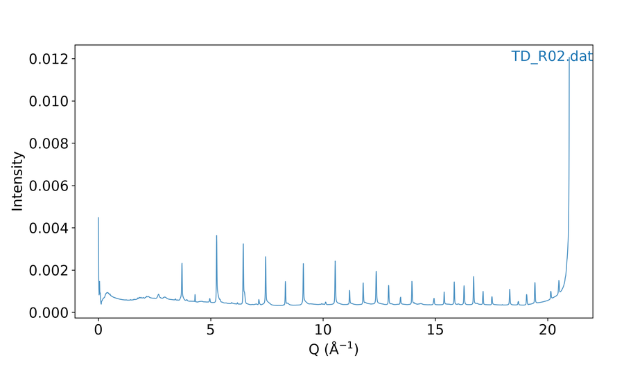
Figure: --readcol 1 3 (TD_R02.dat)

batplot TD_R02.dat --readcol 1 2 1 3 --xaxis q --i

plots two curves: column 1 vs 2, and column 1 vs 3

batplot TD_R02.dat --readcol 1 2-3 --xaxis q --i

same as above using range shorthand for the y columns

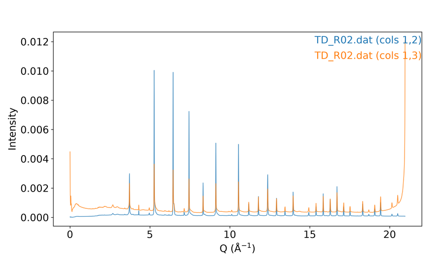
Figure: --readcol 1 2-3 (TD_R02.dat, two y columns)

batplot TD_R02.dat --readcol 1 2 TD_R03.dat --readcol 1 3 --xaxis q --i

per-file column selection when overlaying multiple files

Stacking Multiple Files Using --stack

batplot TD_R02.dat TD_R03.dat --xaxis 2theta --stack --i

batplot (your/optional/path) allfiles --stack --wl 0.259 --i

with allfiles keyword, batplot reads every text/Excel file in the directory, sorts them in natural order (scan2 before scan10), converts them to Q-space using the per-file wavelength, and stacks them vertically.

batplot TD_R02.dat TD_R03.dat TD_R05.dat --stack --wl 0.259 --i

three synchrotron .dat patterns stacked after Q conversion (λ = 0.259 Å)

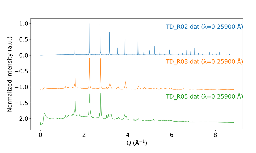
Figure: 1D stack (TD_R02/R03/R05, --stack --wl 0.259)

Plot with CIF Ticks

batplot TD_S0062-64.xy Li2FeSeO.cif --wl 1.54 --i

plots XRD data with CIF ticks in Q space

batplot TD_S0062-64.xy Li2FeSeO.cif:1.54 --xaxis 2theta --wl 1.54 --i

plots XRD data with CIF ticks in 2θ space (figure in Wavelength Handling)

batplot TD_S0062-64.xy:1.54 TD_R02.dat:0.259 Li2FeSeO.cif Li2Se.cif --stack --i

stacks Cu + synchrotron patterns with two CIF tick sets

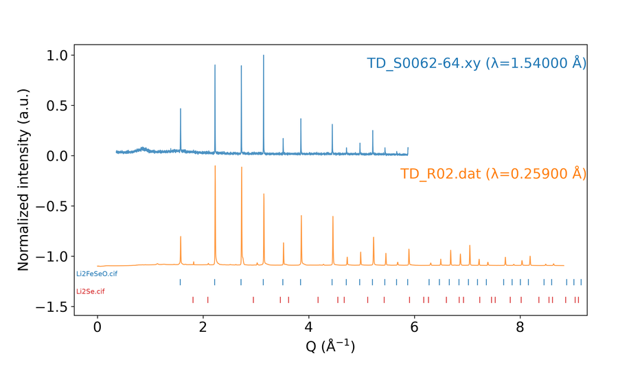
Figure: 1D stack + CIF (Li2FeSeO + Li2Se ticks)

Derivative Plots

The --1d (and --2d) flag plots the first derivative dy/dx of each dataset. This is useful for identifying peak positions and inflection points. The derivative is computed using numpy's gradient function, which handles non-uniform x-spacing automatically.

batplot R03_Se.nor --xaxis energy --i

XAS absorption spectrum

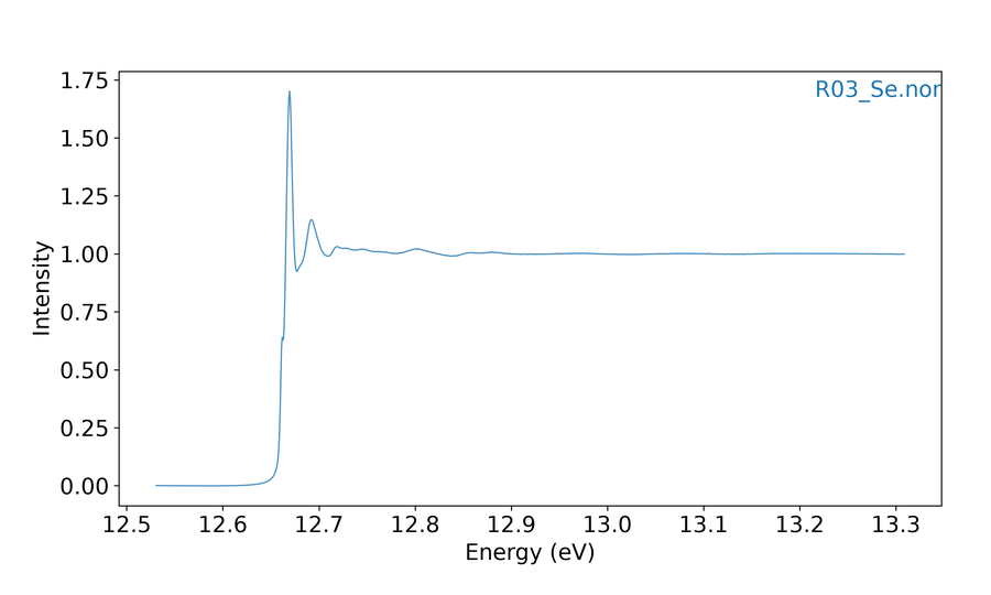
Figure: XAS (R03_Se.nor, --xaxis energy)

batplot R03_Se.nor --1d --xaxis energy --i

first derivative of the XAS spectrum

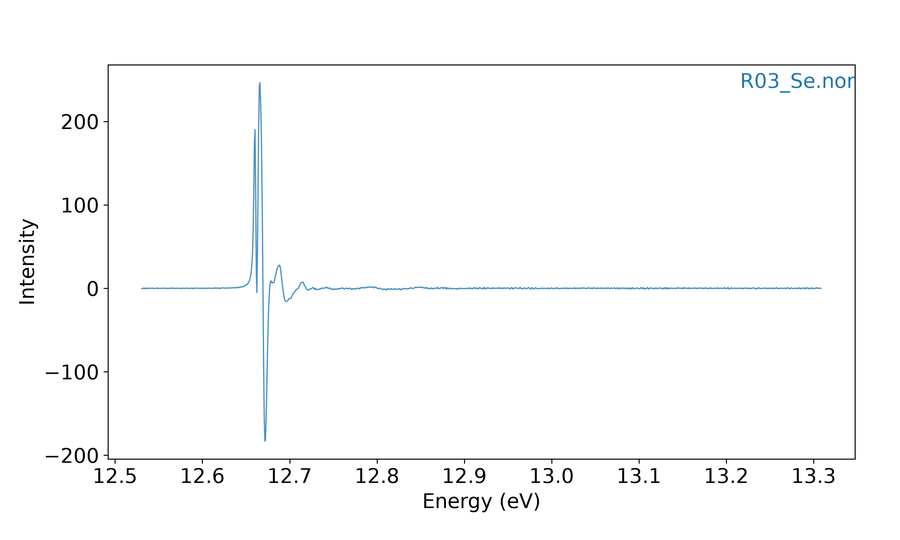
Figure: XAS derivative (--1d --xaxis energy)

batplot allfiles --2d --i

batplot R03_Se.nor --1d --xrange 12600 12700

EXAFS k-Weighting

For EXAFS data in k-space, k-weighting options are available:

Flag

Transformation / use case

--chik

χ(k): standard oscillations

--kchik

k × χ(k): emphasize mid-k features

--k2chik

k² × χ(k): most common weighting, balances signal

--k3chik

k³ × χ(k): emphasize high-k and heavy backscatterers

batplot data.txt --k2chik --i

batplot file1.chik file2.chik --k2chik --stack --i

Batch export (--all)

To export one figure per file in the current folder (SVG by default under Figures/), use --all. Full behavior for XY, EC, histogram, styles, and --all vs allfiles is in Batch mode — --all.

batplot --all --xaxis 2theta

batplot --all mystyle.bpsg

Dual Axes Mode

Use --ry so selected files plot on the right y-axis (--ry disables --stack):

batplot TD_R02.dat TD_R03.dat --ry --wl 0.259 --i

plots TD_R03.dat against the right y-axis

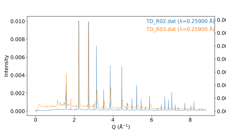
Figure: dual y-axis (TD_R02 + TD_R03 --ry --wl 0.259)

batplot file1.xy file2.xy --ry file3.xy --ry --xaxis 2theta --i

multi-file support for the right y-axis

With --txaxis, right-y curves use the top x-axis (default is a shared bottom x):

batplot file1.xy --ry file2.xy --txaxis --i

Interactive menu (1D / XY) — every key and subkey

Clickable interactive menu

------------------------------------------------------------

1D Interactive Menu:

Styles

c: colors f: font l: line style t: spines/ticks g: size h: legend sm: smooth

Geometries

a: rearrange o: offset r: rename x: change X y: change Y d: derivative cif: CIF ticks

Options

v: find peaks n: crosshair u: axis units (XRD only) p: print(export) style/geom i: import style/geom e: export figure s: save project b: undo q: quit

------------------------------------------------------------

Looks like the live terminal menu. Click a cyan key to jump to its docs. Keys o/y/d hide under --stack; n/u hide for non-XRD.

Add --i to open the 1D Interactive Menu beside the live figure. Type a key, then press Enter. The menu has three columns: Styles | Geometries | Options.

batplot TD_S0062-64.xy:1.54 --i

Key c — Colors

↑ Back to interactive menu

Type a color command at the prompt (not only single letters). Examples: 1:red, all viridis, s:black.

Key / input	What it does	Example
N:color	Set curve number N to a color (name or #RRGGBB).	Type 1:red or 2:#1f77b4.
all palette or 1-3 palette	Apply a colormap to all curves, or only to a numbered range.	Type all viridis or 1-3 plasma.
w:color / a:color / s:color / d:color	Color the top / left / bottom / right spine Use the matching single-key rows for full detail.	Type one option from w:color/a:color/s:color/d:color, for example the first key listed.
t	Show or hide the legend (or enter the legend submenu when nested).	Type t to toggle; if a submenu opens, use p to move it.
v	Print the current color assignments for curves or spines.	Type v to list colors, then adjust with 1:red or s:black.
u	Open the saved-custom-colors helper (store/reuse hex or named colors).	Type u, save a color, then reuse it later as 1:#1f77b4.
e	Pick a color from the screen/eyedropper when the prompt offers it.	Type e, click a pixel on the figure, confirm the hex value.
q	Leave this submenu and return one level up (or to the main menu).	Type q.

---

Key f — Font

↑ Back to interactive menu

Key	What it does	Example
f	Choose font family (pick a number from the list, or type a font name)	Type f, then 1 for the first listed family, or type Arial.
s	Set the font size used for labels and titles.	Type s, then 14.
b	Set weight: type bold or normal, or press Enter to toggle	Type b, then bold (or press Enter to toggle).
h	Open text-highlight settings (box behind labels) — see table below	Type h, then t to turn highlight on.
q	Leave this submenu and return one level up (or to the main menu).	Type q.

Inside h (text highlight):

Key	What it does	Example
t	Turn the text-highlight background box on or off.	Type t.
c	Set the highlight background color behind labels.	Type c, then yellow (or e to pick from the screen).
a	Set highlight transparency from 0 (invisible) to 1 (solid).	Type a, then 0.35.
p	Set how much padding the highlight box adds around text.	Type p, then 0.3.
q	Leave this submenu and return one level up (or to the main menu).	Type q.

---

Key l — Line style

↑ Back to interactive menu

Key	What it does	Example
c	Set the linewidth of the plotted data curves.	Type c, then 1.5.
f	Set linewidth of the axes frame and tick marks.	Type f, then 1.0.
g	Turn the plot grid on/off and adjust grid width when asked.	Type g, then follow the on/off or width prompt.
l	Draw data as solid lines only (no markers).	Type l.
ld	Draw curves as a solid line with markers.	Type ld.
d	Draw markers only (no connecting line) for the selected curves.	Type d (or ld/dd siblings) to switch style, then q back.
da	Draw curves as dashed lines.	Type da.
dd	Draw curves as dashed lines with markers.	Type dd.
q	Leave this submenu and return one level up (or to the main menu).	Type q.

---

Key t — Spines and ticks (WASD)

↑ Back to interactive menu

Spines are the four border lines of the axes box. Tick marks, tick numbers, and axis titles sit on those sides.

Press t, then type commands at the spine prompt. Most toggles are a side letter + number with no space (for example s2). You can put several codes on one line.

Step 1 — Pick a side (WASD)

Key	What it does	Example
w	WASD top side of the axes box.	Type w5 to toggle the top axis title.
a	WASD left side of the axes box.	Type a4 to toggle left tick numbers.
s	WASD bottom side of the axes box.	Type s2 to toggle bottom major ticks.
d	WASD right side of the axes box.	Type d1 to toggle the right spine line.

Step 2 — Pick what to show/hide on that side

Number	What it does	Example
1	Toggle the border spine line on the chosen side.	s1 toggles the bottom spine.
2	Toggle major tick marks on the chosen side.	a2 toggles left major ticks.
3	Toggle minor tick marks on the chosen side.	s3 toggles bottom minor ticks.
4	Toggle tick number labels on the chosen side.	a4 hides or shows left numbers.
5	Toggle the axis title on the chosen side.	w5 toggles the top title.

Examples (copy these ideas)

You type	What it does	Example
s2	Toggle bottom major tick marks on the plot frame.	Type s2 once to hide bottom majors; type again to show them.
w5	Toggle the top axis title visibility.	Type w5 to hide the top title if it overlaps the plot.
a4	Toggle left-side tick number labels.	Type a4 to hide left numbers for a cleaner export.
d1	Toggle the right spine (border) line.	Type d1 to remove the right border.
s2 w5 a4	Apply several WASD toggles in one command (space-separated).	Type s2 w5 a4 to hide bottom majors, top title, and left numbers together.

Blank line or q leaves a nested prompt; q on the spine prompt returns to the main interactive menu.

Extra commands (type the letter alone)

Key	What it does	How to use it	Example
i	Flip tick marks to point into vs out of the plot.	Type i once; type again to flip back	Type i once; type again to flip back.
l	Set major tick length (points). Minor length is set automatically to about 70%	Type l, then enter a positive number	Type l, then 6.
n	Set spacing between major ticks.	Type n, then e.g. x 0.5, y 1, all 1, or x auto	Type n, then x 0.5, all 1, or x auto.
m	Set how many minor ticks sit between majors.	Type m, then e.g. x 4 or all 0 (off)	Type m, then x 4 or all 0 to disable.
p	Nudge axis titles away from the data.	See the next table	Type p, then w and use nudge keys.
list	Print the current spine/tick on/off state for every side.	Read the report, then continue	Type list.
q	Leave this submenu and return one level up (or to the main menu).	Back to the main interactive menu	Type q.

Inside p — move axis titles

Key	What it does	Example
w	WASD top side of the axes box.	Type w5 to toggle the top axis title.
s	WASD bottom side of the axes box.	Type s2 to toggle bottom major ticks.
a	WASD left side of the axes box.	Type a4 to toggle left tick numbers.
d	WASD right side of the axes box.	Type d1 to toggle the right spine line.
r	Reset all title-offset nudges back to the default positions.	Type r after overshooting with x 0.5 / y -0.3.
q	Leave this submenu and return one level up (or to the main menu).	Type q.

Typical nudge keys after you pick a side: w/s/a/d to move, 0 to reset that title, q to go back.

Workflow tip

1. Press t on the main menu.
2. Toggle borders/ticks with codes like s2 until the frame looks right.
3. Use n / m so tick spacing matches your data range.
4. Use p if a title sits too close to the data.
5. Press q to return to the main menu (your figure stays updated).

---

Key g — Size

↑ Back to interactive menu

Press g, then choose what to resize. Sizes are in inches.

Key	What it does	Example
p	Resize the axes box (plot frame) in inches.	Type p, then 6 4.
c	Resize the whole figure window in inches.	Type c, then 8 6.
q	Leave this submenu and return one level up (or to the main menu).	Type q.

How to enter a size: after p or c, type two numbers such as 6 4 (width height), or follow the printed prompt. Soft quit with q / blank if you change your mind — you should not get an “invalid size” error for quitting.

---

Key h — Legend

↑ Back to interactive menu

Key	What it does	Example
v	Show or hide curve names inside the legend.	Type v.
s	Move the legend to a corner.	Type s, then 1 (top-right).
q	Leave this submenu and return one level up (or to the main menu).	Type q.

Inside s (legend position):

Key	What it does	Example
1	Place the legend in the top-right corner.	Type 1.
2	Place the legend in the top-left corner.	Type 2.
3	Place the legend in the bottom-right corner.	Type 3.
4	Place the legend in the bottom-left corner.	Type 4.

---

Key sm — Smooth / reduce

↑ Back to interactive menu

Use this to thin noisy data or apply a smoother. Press sm on the main menu first.

Key	What it does	Example
r	Open tools that thin the number of points.	Type r, then 1 for delete-N / skip-M.
s	Open smoothing filters for the curves.	Type s, then 2 for Savitzky–Golay.
reset	Restore data from before the last transform in this menu.	Type reset.
q	Leave this submenu and return one level up (or to the main menu).	Type q.

After you press r (reduce points):

Key	What it does	Example
1	Keep the first value in each grouped bin.	Type 1 after setting the group size.
2	Keep the last value in each grouped bin.	Type 2.
3	Average values within each grouped bin.	Type 3.
q	Leave this submenu and return one level up (or to the main menu).	Type q.

After you press r, then 3 (merge rule):

Key	What it does	Example
1	Keep the first value in each grouped bin.	Type 1 after setting the group size.
2	Keep the last value in each grouped bin.	Type 2.
3	Average values within each grouped bin.	Type 3.
4	Keep the minimum in each grouped bin.	Type 4.
5	Keep the maximum in each grouped bin.	Type 5.
6	Sum values within each grouped bin.	Type 6.

After you press s (smooth):

Key	What it does	Example
1	Keep the first value in each grouped bin.	Type 1 after setting the group size.
2	Keep the last value in each grouped bin.	Type 2.
3	Average values within each grouped bin.	Type 3.
q	Leave this submenu and return one level up (or to the main menu).	Type q.

---

Key a — Rearrange curves

↑ Back to interactive menu

No letter submenu. The menu lists curves as 1, 2, 3, …. Type a new order with spaces, for example 3 1 2 4.

If the plot becomes messy after reordering, prefer launching with --stack.

---

Key o — Vertical offset

↑ Back to interactive menu

Not available when you used --stack.

Key	What it does	Example
1 … N	Pick which curve number to vertically offset.	Type 1, then enter an offset such as 0.2.
a	Set equal spacing between stacked curves (prompts for the gap).	Type a, then 0.15 to space curves by 0.15 intensity units.
r	Reset all curve offsets back to 0.	Type r to collapse every curve to its original baseline.
d	Change the default delta spacing used when applying offsets (original stack spacing).	Type d, then 0.2 to set the spacing step.
q	Leave this submenu and return one level up (or to the main menu).	Type q.

---

Key r — Rename

↑ Back to interactive menu

Key	What it does	Example
c	Rename one plotted curve in the legend.	Type c, pick curve 1, then enter Sample A.
t	Rename a CIF phase title (only if CIF ticks are loaded).	Type t, pick the phase, then enter Li$_2$Se.
x	Set the X-axis title text (use m first if you need math syntax help).	Type x, then 2$\theta$ (deg) or Q (Å$^{-1})$.
y	Set the Y-axis title text.	Type y, then Intensity (a.u.).
s	Show recently used titles and optionally reuse one.	Type s, then enter 1 to reuse the first recent title.
m	Show help for subscripts, superscripts, and Greek letters in titles.	Type m, read the help, then rename with {sub(2)} / Greek tokens.
q	Return to the main interactive menu.	Type q.

---

Key x / y — Axis limits

↑ Back to interactive menu

Same controls for X (x) and Y (y). Y is hidden with --stack.

Key / input	What it does	Example
min max	Enter both limits as two numbers separated by a space.	10 80 or 3.0 4.2.
w	Raise/step the upper axis limit.	Type w a few times, or enter a numeric max when prompted.
s	Lower/step the lower axis limit (pair with w for the upper).	Type s a few times, or enter a numeric min when prompted.
a	Auto-scale this axis to the visible data.	Type a after zooming too far.
q	Leave this submenu and return one level up (or to the main menu).	Type q.

---

Key d — Derivative

↑ Back to interactive menu

Not available with --stack.

Key	What it does	Example
1	Compute dy/dx for the curves.	Type 1.
2	Compute the second derivative.	Type 2.
3	Compute the reversed derivative dx/dy.	Type 3.
4	Compute the reversed second derivative.	Type 4.
reset	Restore data from before the last transform in this menu.	Type reset.
q	Leave this submenu and return one level up (or to the main menu).	Type q.

---

Key cif — CIF reference ticks

↑ Back to interactive menu

If no CIF is loaded yet:

Key	What it does	Example
a	Add a CIF (or add files — follow this menu’s label).	Type a, then Li2Se.cif.
q	Leave this submenu and return one level up (or to the main menu).	Type q.

After at least one CIF set exists:

Key	What it does	Example
a	Add one or more CIF files as reference tick sets.	Type a, then Li2Se.cif.
z	Toggle Miller-index (hkl) labels on CIF ticks.	Type z to show or hide hkl text.
t	Toggle CIF phase titles on/off.	Type t if titles crowd the plot.
v	Change the vertical order of CIF tick rows.	Type v, then enter a new sequence of set numbers.
p	Shift all CIF ticks up/down (w/s or a numeric value).	Type p, then w or 0.05.
c	Set CIF tick colors per set.	Type c, pick set 1, then red or #1f77b4.
x	Show or hide one CIF tick set.	Type x, then the set number.
r	Rename a CIF phase label (same idea as main-menu r → t).	Type r, pick the set, then enter Li$_2$Se.
q	Return to the main interactive menu.	Type q.

---

Key v — Find peaks

↑ Back to interactive menu

Key / input	What it does	Example
min max	Enter both limits as two numbers separated by a space.	10 80 or 3.0 4.2.
current	Use the current on-screen axis window as the search range.	Type current.
q	Leave this submenu and return one level up (or to the main menu).	Type q.

Follow any further numeric prompts (threshold, etc.) as printed.

---

Key n — Crosshair

↑ Back to interactive menu

Only on diffraction plots. Press n to turn the mouse crosshair on; press n again to turn it off. Move the mouse over the plot to read coordinates.

---

Key u — Axis units (XRD only)

↑ Back to interactive menu

Converts the live X-axis between 2θ and Q. Hidden for non-XRD data (PDF, XAS, custom axes). Switching that involves 2θ needs a wavelength (--wl, file:wl, or a prompt). This does not write a new data file — use --convert for export.

Key	What it does	Example
2	Convert the live X-axis to 2θ (deg).	Type 2 (enter λ if prompted).
q	Convert the live X-axis to Q (Å⁻¹).	Type q.
b	Go back without changing the axis.	Type b.

Data, axis labels/limits, and CIF ticks stay in sync after conversion.

Keys p / i / e / s / b / q — Save, style, export

↑ Back to interactive menu

Key	What it does	Example
p	Export style: usually choose style only (.bps) or style + geometry (.bpsg)	Type p, choose style-only or style+geometry.
i	Import a saved style by picking its number from the list.	Type i, then 2.
e	Export overview values to a file.	Type e.
s	Save the session as a .pkl file.	Type s, then confirm the name/folder.
b	Undo the last change stored in history.	Type b.
q	Quit the interactive menu (save first if you need the session)	Type q.

Convert and export XRD data files

Plot-time conversion (--wl, :λ, interactive u) only changes what you see. To write converted columns for Origin, Rietveld software, or another pipeline, use --convert. Originals are never modified; outputs go into a converted/ subfolder next to each input.

batplot TD_S0062-64.xy --convert 1.54 q

2θ (Cu) → Q → converted/TD_S0062-64.qye

batplot TD_S0062-64.xy --convert 1.54 0.709

re-project 2θ from Cu λ to Mo-like λ → converted/… .xy

batplot TD_R02.dat --readcol 1 2 --convert 0.259 q

choose columns, then export Q

batplot allfiles --ext xy --convert 2theta q --wl 1.54 --convert-ext qye

batch-convert every .xy in the folder

Full conversion matrix (2θ ↔ Q ↔ d), --ext / --convert-ext, and folder workflows: Utilities — Convert XRD files.