6. Electrochemistry (EC) and CPC / EPC Modes¶

Electrochemistry mode supports four visualization types: galvanostatic cycling (GC), cyclic voltammetry (CV), differential capacity (dQ/dV), and capacity/energy density-per-cycle (CPC). Both Biologic (.mpt) and Neware (.csv) files are read directly. More instruments are supported upon request.

Requirement for data exporting from instruments:

Neware: Customizer report – check all boxes – export to .csv or .xlsx format

BioLogic: Export all to .mpt file

Note

For BioLogic .mpt files in GC and CPC modes, pass --mass in milligrams (or with a g suffix for grams). For Neware .csv/.xlsx files that already store specific capacity, --mass is usually not needed. If the Neware export only has absolute capacity, you still need --mass to get mAh/g.

Galvanostatic Cycling (GC)¶

Plot potential vs. specific capacity charge/discharge profiles:

batplot B443.csv --gc --i

from a Neware .csv file

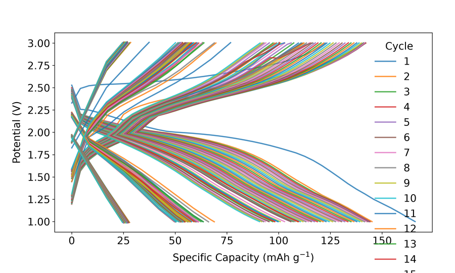
Figure: GC mode (B443.csv --gc)

batplot TD_O2.mpt --gc --mass 7.0 --i

from a Biologic .mpt file (mass required in milligrams)

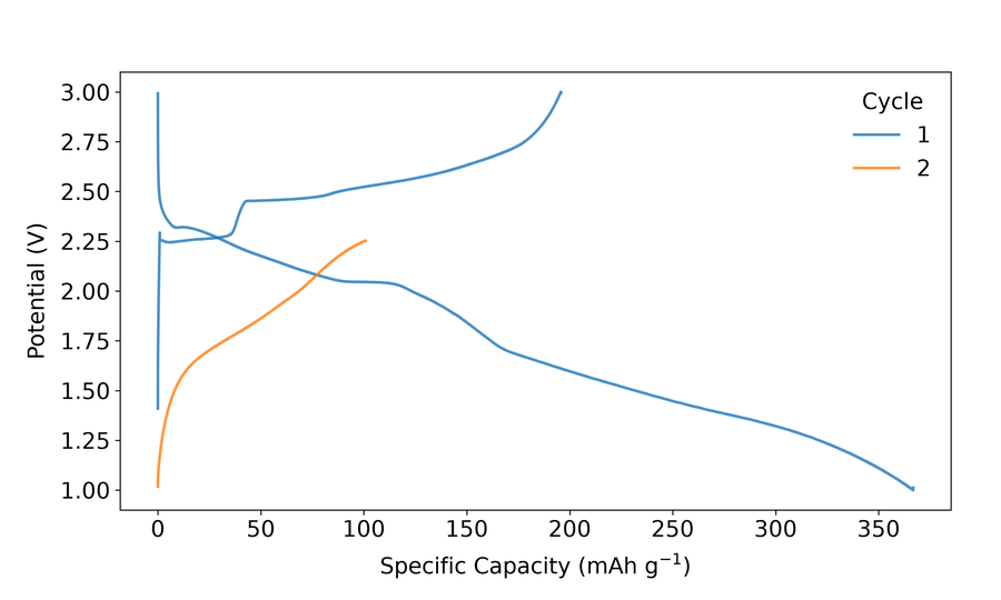
Figure: GC from Biologic (TD_O2.mpt --gc --mass 7)

batplot battery.mpt --gc --mass 12g --i

from a Biologic .mpt file with high mass loading in grams

batplot B443.csv B444.csv B445.csv --gc --i

plots all three Neware files

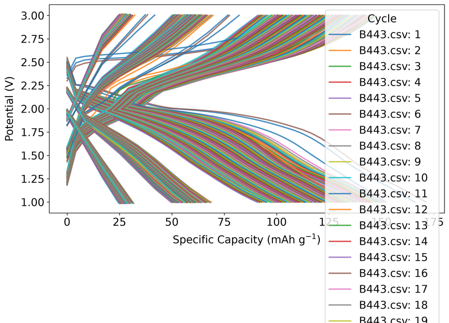
Figure: multi-file GC (B443 + B444 + B445)

Cyclic Voltammetry (CV)¶

Plot current vs. voltage cycles for electrochemical characterization:

batplot cyclic.mpt --cv --i

Differential Capacity (dQ/dV)¶

Plot dQ/dV vs. potential to identify electrochemical reaction peaks:

batplot B443.csv --dqdv --i

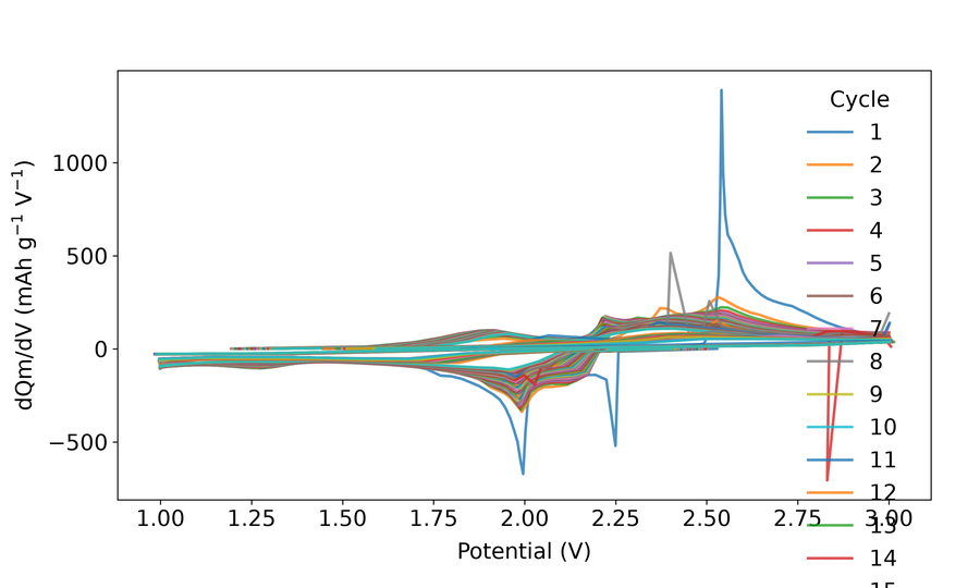
Figure: dQ/dV (B443.csv --dqdv)

batplot B443.csv B444.csv --dqdv --i

plots multiple files and compare the peaks

Capacity Per Cycle (CPC)¶

CPC mode plots charge and discharge specific capacity (and optionally coulombic efficiency) as a function of cycle number. Multiple files from different samples can be overlaid on the same figure.

batplot B443.csv --cpc --i

single file

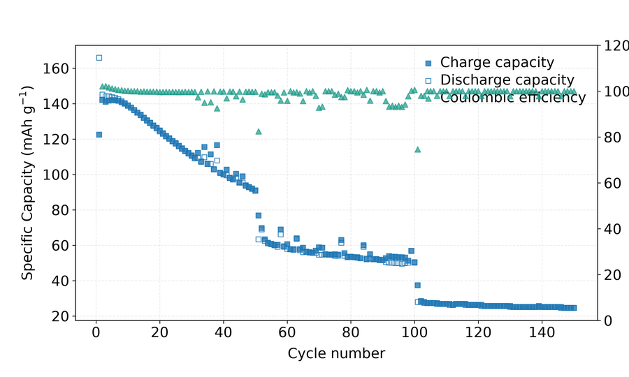
Figure: CPC mode (B443.csv --cpc)

batplot B443.csv B444.csv B445.csv --cpc --i

multiple Neware files overlaid in CPC mode

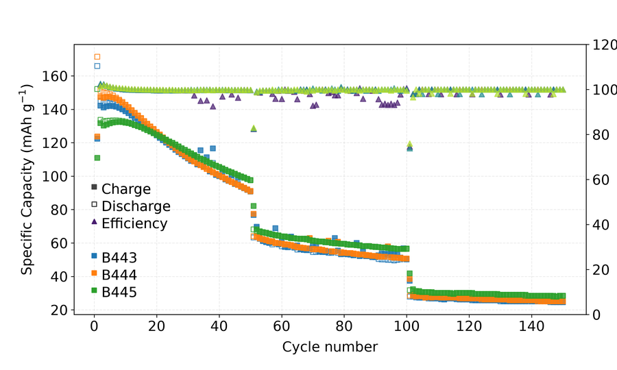
Figure: multi-file CPC (B443 + B444 + B445)

batplot file1.csv file2.mpt --mass 6.0 --cpc --i

multiple files from different instruments

Time vs. Voltage¶

Plot the raw time (hours) vs. voltage profile from a CSV or MPT file:

batplot B443.csv --xaxis time --i

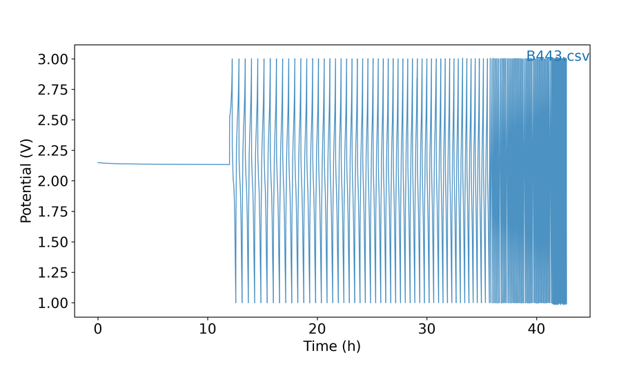
Figure: time vs voltage (B443.csv --xaxis time)

Add --i with --gc, --cv, or --dqdv. Type a key, then press Enter. Columns: Styles | Geometries | Options. Some keys appear only for certain plot types.

Key	What it does	Example
`f`	Choose font family (number from the list, or type a name)	Type `f`, then `1` for the first listed family, or type `Arial`.
`s`	Set the font size used for labels and titles.	Type `s`, then `14`.
`b`	Set bold vs normal weight (blank Enter often toggles).	Type `b`, then `bold` (or press Enter to toggle).
`h`	Open text-highlight tools (colored box behind label text).	Type `h`, then `t` to turn highlight on.
`q`	Leave this submenu and return one level up (or to the main menu).	Type `q`.

Key	What it does	Example
`t`	Turn the text-highlight background box on or off.	Type `t`.
`c`	Set the highlight background color behind labels.	Type `c`, then `yellow` (or `e` to pick from the screen).
`a`	Set highlight transparency from 0 (invisible) to 1 (solid).	Type `a`, then `0.35`.
`p`	Set how much padding the highlight box adds around text.	Type `p`, then `0.3`.
`q`	Leave this submenu and return one level up (or to the main menu).	Type `q`.

Key	What it does	Example
`c`	Set the linewidth of the plotted data curves.	Type `c`, then `1.5`.
`f`	Set linewidth of the axes frame and tick marks.	Type `f`, then `1.0`.
`g`	Turn the plot grid on/off and adjust grid width when asked.	Type `g`, then follow the on/off or width prompt.
`l`	Draw data as solid lines only (no markers).	Type `l`.
`ld`	Draw curves as a solid line with markers.	Type `ld`.
`d`	Draw markers only (no connecting line) for the selected curves.	Type `d` (or `ld`/`dd` siblings) to switch style, then `q` back.
`da`	Draw curves as dashed lines.	Type `da`.
`dd`	Draw curves as dashed lines with markers.	Type `dd`.
`q`	Leave this submenu and return one level up (or to the main menu).	Type `q`.

Key	What it does	Example
`a`	Potential-step filter — follows numeric prompts; type `e` at a prompt if you want an on-screen explanation	Type `a`, then enter parameters (or `e` for explain).
`d`	Apply the DiffCap filter on dQ/dV.	Type `d`, then follow prompts.
`o`	Open outlier-removal methods.	Type `o`, then `1` or `2`.
`r`	Reset filtered dQ/dV data back to the original curves.	Type `r` after a filter that removed too much.
`q`	Leave this submenu and return one level up (or to the main menu).	Type `q`.

Key	What it does	Example
`1`	Remove outliers with a Z-score rule.	Type `1`, then follow the threshold prompt.
`2`	Remove outliers with median absolute deviation (MAD).	Type `2`.

Key / input	What it does	Example
`w:color`	Set the top spine color (name or `#RRGGBB`).	Type `w:black` or `w:#333333`.
`a:color`	Set the left spine color.	Type `a:red` to match a left-axis series.
`s:color`	Set the bottom spine color.	Type `s:#444444`.
`d:color`	Set the right spine color.	Type `d:blue` when a right axis is used.
`e`	Pick a color from the screen/eyedropper when the prompt offers it.	Type `e`, click a pixel on the figure, confirm the hex value.
`u`	Open the saved-custom-colors helper (store/reuse hex or named colors).	Type `u`, save a color, then reuse it later as `1:#1f77b4`.
`q`	Leave this submenu and return one level up (or to the main menu).	Type `q`.

Key	What it does	Example
`w`	WASD top side of the axes box.	Type `w5` to toggle the top axis title.
`a`	WASD left side of the axes box.	Type `a4` to toggle left tick numbers.
`s`	WASD bottom side of the axes box.	Type `s2` to toggle bottom major ticks.
`d`	WASD right side of the axes box.	Type `d1` to toggle the right spine line.

Number	What it does	Example
`1`	Toggle the border spine line on the chosen side.	`s1` toggles the bottom spine.
`2`	Toggle major tick marks on the chosen side.	`a2` toggles left major ticks.
`3`	Toggle minor tick marks on the chosen side.	`s3` toggles bottom minor ticks.
`4`	Toggle tick number labels on the chosen side.	`a4` hides or shows left numbers.
`5`	Toggle the axis title on the chosen side.	`w5` toggles the top title.

You type	What it does	Example
`s2`	Toggle bottom major tick marks on the plot frame.	Type `s2` once to hide bottom majors; type again to show them.
`w5`	Toggle the top axis title visibility.	Type `w5` to hide the top title if it overlaps the plot.
`a4`	Toggle left-side tick number labels.	Type `a4` to hide left numbers for a cleaner export.
`d1`	Toggle the right spine (border) line.	Type `d1` to remove the right border.
`s2 w5 a4`	Apply several WASD toggles in one command (space-separated).	Type `s2 w5 a4` to hide bottom majors, top title, and left numbers together.

Key	What it does	How to use it	Example
`i`	Flip tick marks to point into vs out of the plot.	Type `i` once; type again to flip back	Type `i` once; type again to flip back.
`l`	Set major tick length (points). Minor length is set automatically to about 70%	Type `l`, then enter a positive number	Type `l`, then `6`.
`n`	Set spacing between major ticks.	Type `n`, then e.g. `x 0.5`, `y 1`, `all 1`, or `x auto`	Type `n`, then `x 0.5`, `all 1`, or `x auto`.
`m`	Set how many minor ticks sit between majors.	Type `m`, then e.g. `x 4` or `all 0` (off)	Type `m`, then `x 4` or `all 0` to disable.
`p`	Nudge axis titles away from the data.	See the next table	Type `p`, then `w` and use nudge keys.
`list`	Print the current spine/tick on/off state for every side.	Read the report, then continue	Type `list`.
`q`	Leave this submenu and return one level up (or to the main menu).	Back to the main interactive menu	Type `q`.

Situation	What it does	Example
Normal GC / CV / dQ/dV	`n` and `m` prompts usually offer `x`, `y`, and `all` Use the matching single-key rows for full detail.	Type one option from Normal GC / CV / dQ/dV, for example the first key listed.
Dual-X GC (capacity + ions)	Spacing prompts may also offer `tx` for the top X axis — use `tx 0.5` the same way as `x 0.5`.	After enabling dual-X, type `t` → spacing → `tx 0.4` to nudge the top X title.
After changing cycles or dual axis	Re-open `t` if tick spacing looks stale; `n`/`m` re-apply cleanly.	Change cycles, then type `t` and set major spacing again if labels look wrong.

Step	What it does	Example
1	From the dQ/dV interactive menu, press `2d` to open a contour companion.	Type `2d` on the dQ/dV menu.
2	Enter the potential window when asked (min and max V).	When prompted, type `2.5 4.2`.
3	Style the new contour window (colormap, ranges, export, …).	In the contour menu, type `oc` then `viridis`.
4	Save that contour with `s` if you want a `.pkl` for later / batch styling.	Type `s`, choose a path, confirm.

Tip	What it does	Example
Efficiency axis	After showing efficiency with `ry`, you may want `d2` / `d4` (right ticks/labels) visible.	Type `ry` to show efficiency, then `d4` so right-axis numbers appear.
Spine colors	Use main-menu `k` or `c` → `s`, not the `t` (ticks) menu.	Type `k`, then `a:black` to color the left spine.

Key	What it does	Example
`p`	Set the plot frame (axes box) width × height — enter two numbers such as `6 4`	Type `p`, then `6 4`.
`c`	Resize the whole figure window in inches.	Type `c`, then `8 6`.
`q`	Leave this submenu and return one level up (or to the main menu).	Type `q`.

Key	What it does	Example
`t`	Show or hide the legend.	Type `t` to toggle the legend on/off.
`p`	Open legend-position controls.	Type `p`, then `w`/`s` or `0.1 0.9`.
`ra`	Reorder legend entries when several files are plotted.	Type `ra`, then `2 1 3`.
`q`	Leave this submenu and return one level up (or to the main menu).	Type `q`.

Key / input	What it does	Example
`w` / `s` / `a` / `d`	Nudge the legend Use the matching single-key rows for full detail.	Type one option from w`/`s`/`a`/`d, for example the first key listed.
`0`	Reset the legend (or item) position to the default.	Type `0` after moving the legend off-canvas.
`x` / `y`	Lock motion to one axis Use the matching single-key rows for full detail.	Type one option from x`/`y, for example the first key listed.
`x y`	Set an absolute legend position with two numbers (axes fraction).	Type `0.02 0.98` for upper-left inside the axes.
`q`	Leave this submenu and return one level up (or to the main menu).	Type `q`.

Key	What it does	Example
`c`	Show charge half-cycles only.	Type `c`.
`d`	Show discharge half-cycles only.	Type `d`.
`b`	Show both charge and discharge traces.	Type `b`.
`q`	Leave this submenu and return one level up (or to the main menu).	Type `q`.

Key	What it does	Example
`1` … `N`	Select that file number to edit cycles or colors.	Type `1`, then set cycles like `1-10` or a color.
`v`	Print the current color assignments for curves or spines.	Type `v` to list colors, then adjust with `1:red` or `s:black`.
`q`	Leave this submenu and return one level up (or to the main menu).	Type `q`.

Input	What it does	Example
`1-5` or `all`	Select which cycles to show or restyle.	Type `1-5` for cycles 1–5, or `all` for every cycle.
`1:red`	Set the color of one cycle (name or `#RRGGBB`).	Type `3:blue` or `2:#d62728`.
`all viridis`	Apply a colormap across the selected / all cycles.	Type `all viridis` or `1-10 plasma`.
`fall:…`	Fall-related helpers when the menu offers them (e.g. fall coloring).	Type the printed `fall:…` form if shown.
`v`	Print the current cycle colors.	Type `v`, read the list, then adjust with `1:red`.
`e`	Pick a color from the screen for the active cycle/file.	Type `e`, click a pixel, confirm.
`u`	Reuse a saved custom color.	Type `u`, pick a saved entry, apply it.
`q`	Leave this cycle/color prompt.	Type `q`.

Key	What it does	Example
`x`	Set the bottom X-axis title (usually capacity, or time in time-mode plots).	Type `x`, then `Capacity (mAh g$^{-1}$)`.
`tx`	Set the top X-axis title when dual-X (capacity + ions) is enabled.	Type `tx`, then `x in Li$_x$MO$_2$`.
`y`	Set the Y-axis title (usually potential).	Type `y`, then `Potential (V vs Li/Li$^+$)`.
`f`	Rename a file entry in the legend (multi-file sessions).	Type `f`, pick file `2`, then enter `Cell B`.
`s`	Show recently used titles and optionally reuse one.	Type `s`, then enter `1`.
`m`	Show math / Greek typing help for titles.	Type `m`, then use `{sub(2)}` when renaming.
`q`	Return to the main EC menu.	Type `q`.

Key	What it does	Example
`c`	Show capacity only on the bottom X-axis.	Type `c` to leave ions/dual mode and plot capacity.
`n`	Show number of ions only on the bottom X-axis.	Type `n` (needs mass / capacity-per-ion params when prompted).
`d`	Enable dual X-axis (capacity bottom, ions top).	Type `d` to show both scales at once.
`s`	Swap top and bottom axes while in dual mode.	Type `s` after `d` to put ions on the bottom.
`u`	Update the theoretical capacity / ion-conversion parameters.	Type `u`, then enter new mass or capacity-per-ion values.
`q`	Return to the main EC menu.	Type `q`.

Key / input	What it does	Example
`min max`	Enter both limits as two numbers separated by a space.	`10 80` or `3.0 4.2`.
`w`	Raise/step the upper axis limit.	Type `w` a few times, or enter a numeric max when prompted.
`s`	Lower/step the lower axis limit.	Type `s` a few times, or enter a numeric min when prompted.
`a`	Auto-scale this axis to the visible data.	Type `a` after zooming too far.
`q`	Leave this submenu and return one level up (or to the main menu).	Type `q`.

Key	What it does	Example
`c`	Open the capacity / efficiency summary table.	Type `c`, inspect printed values, then `q` back.
`r`	Open the retention overview table.	Type `r`.
`s`	Show a short numerical summary of the overview.	Type `s`.
`e`	Export overview values to a file.	Type `e`.
`q`	Leave this submenu and return one level up (or to the main menu).	Type `q`.

6. Electrochemistry (EC) and CPC / EPC Modes¶

Galvanostatic Cycling (GC)¶

Cyclic Voltammetry (CV)¶

Differential Capacity (dQ/dV)¶

Capacity Per Cycle (CPC)¶

Time vs. Voltage¶

Interactive menu — Electrochemistry (GC / CV / dQ/dV)¶

Clickable interactive menu¶

Key f — Font¶

Key l — Line style¶

Key sm — Smooth / filter (dQ/dV only)¶

Key k — Spine colors¶

Key t — Spines and ticks¶

Step 1 — Pick a side (WASD)¶

Step 2 — Pick what to show/hide on that side¶

Examples (copy these ideas)¶

Extra commands (type the letter alone)¶

Inside p — move axis titles¶

Electrochemistry-specific notes¶

Key g — Size¶

Key h — Legend¶

Key d — Display charge / discharge¶

Key v — Show / hide files¶

Key c — Cycles and colors¶

Key r — Rename¶

Key a — Capacity / ions (GC only)¶

Key x / y — Axis limits¶

Key o — Overview (GC only)¶

Key 2d — dQ/dV contour (dQ/dV only)¶

Keys n / p / i / e / s / b / q¶

Interactive menu — CPC / EPC¶

Clickable interactive menu¶

Key f — Font¶

Key l — Line widths¶

Key m — Marker sizes¶

Key c — Colors¶

Key k — Spine colors¶

Key d — Display Chg / Dch¶

Key ry — Efficiency axis¶

Key t — Spines and ticks¶

Step 1 — Pick a side (WASD)¶

Step 2 — Pick what to show/hide on that side¶

Examples (copy these ideas)¶

Extra commands (type the letter alone)¶

Inside p — move axis titles¶

CPC-specific notes¶

Key h — Legend¶

Key g — Size¶

Key v — Show / hide files¶

Key r — Rename¶

Key x — X limits¶

Key y — Y limits¶

Key ie — Invert efficiency¶

Key a — Add file(s)¶

Key o — Overview¶

Keys n / p / i / e / s / b / q¶

Key `f` — Font¶

Key `l` — Line style¶

Key `sm` — Smooth / filter (dQ/dV only)¶

Key `k` — Spine colors¶

Key `t` — Spines and ticks¶

Inside `p` — move axis titles¶

Key `g` — Size¶

Key `h` — Legend¶

Key `d` — Display charge / discharge¶

Key `v` — Show / hide files¶

Key `c` — Cycles and colors¶

Key `r` — Rename¶

Key `a` — Capacity / ions (GC only)¶

Key `x` / `y` — Axis limits¶

Key `o` — Overview (GC only)¶

Key `2d` — dQ/dV contour (dQ/dV only)¶

Keys `n` / `p` / `i` / `e` / `s` / `b` / `q`¶

Key `f` — Font¶

Key `l` — Line widths¶

Key `m` — Marker sizes¶

Key `c` — Colors¶

Key `k` — Spine colors¶

Key `d` — Display Chg / Dch¶

Key `ry` — Efficiency axis¶

Key `t` — Spines and ticks¶

Inside `p` — move axis titles¶

Key `h` — Legend¶

Key `g` — Size¶

Key `v` — Show / hide files¶

Key `r` — Rename¶

Key `x` — X limits¶

Key `y` — Y limits¶

Key `ie` — Invert efficiency¶

Key `a` — Add file(s)¶

Key `o` — Overview¶

Keys `n` / `p` / `i` / `e` / `s` / `b` / `q`¶

Key	What it does	Example
`n`	Toggle the crosshair helper on the figure.	Type `n` once to show, again to hide.
`p`	Export a reusable style file (`.bps` / `.bpsg` / `.bpsh`).	Type `p`, choose style-only or style+geometry.
`i`	Import a saved style by picking its number from the list.	Type `i`, then `2`.
`e`	Export the figure image (svg, png, …).	Type `e`, choose format and folder.
`s`	Save the session as a `.pkl` file.	Type `s`, then confirm the name/folder.
`b`	Undo the last change stored in history.	Type `b`.
`q`	Leave this submenu and return one level up (or to the main menu).	Type `q`.

Key	What it does	Example
`f`	Choose font family (pick a number from the list, or type a font name)	Type `f`, then `1` for the first listed family, or type `Arial`.
`s`	Set the font size used for labels and titles.	Type `s`, then `14`.
`b`	Set weight: type `bold` or `normal`, or press Enter to toggle	Type `b`, then `bold` (or press Enter to toggle).
`h`	Text highlight (colored box behind labels) — see next table	Type `h`, then `t` to turn highlight on.
`q`	Leave this submenu and return one level up (or to the main menu).	Type `q`.

Prompt (typical)	What it does	Example
Charge markers	A positive size number (matplotlib marker size) for charge points.	Enter `8` for larger charge markers.
Discharge markers	A positive size number for discharge markers.	Enter `6`.
Efficiency markers	A positive size number when efficiency is plotted.	Enter `5`.

Key	What it does	Example
`ly`	Color the left-Y (capacity/energy) curves.	Type `ly`, then `1:red` or a palette command.
`ry`	Color the right-Y (efficiency) series when shown.	Type `ry`, then `green`.
`s`	Open spine-color controls (top/bottom/left/right, optional auto).	Type `s`, then `a:black`.
`u`	Manage saved custom colors for reuse.	Type `u`, save a hex, reuse later.
`e`	Pick a color from the screen/eyedropper.	Type `e`, click a pixel, confirm.
`q`	Return to the main CPC menu.	Type `q`.

Key / input	What it does	Example
`w:color` / `a:color` / `s:color` / `d:color`	Color the top / left / bottom / right spine.	Type `w:black` or `a:#4561F7`.
`auto`	Apply automatic spine/label colors (typically single-file sessions).	Type `auto` to restore default spine coloring.
`e`	Pick a color from the screen/eyedropper when the prompt offers it.	Type `e`, click a pixel on the figure, confirm the hex value.
`q`	Return to the previous menu without further changes.	Type `q`.

Key / input	What it does	Example
`w` / `a` / `s` / `d` (+ color as prompted)	Color the top / left / bottom / right spine.	Type `a` then `red`, or `w:#333333`.
`auto`	Apply automatic spine/label colors (typically single-file sessions).	Type `auto` to restore default spine coloring.
`e`	Pick a color from the screen/eyedropper when the prompt offers it.	Type `e`, click a pixel on the figure, confirm the hex value.
`q`	Return to the previous menu without further changes.	Type `q`.

Key	What it does	Example
`t`	Show or hide the efficiency (right) axis.	Type `t`.
`q`	Return to the previous menu without further changes.	Type `q`.

Key	What it does	Example
`t`	Show or hide the legend box.	Type `t`.
`p`	Open legend-position controls.	Type `p`, then `w`/`s` or `0.1 0.9`.
`ra`	Reorder legend entries when several files are plotted.	Type `ra`, then `2 1 3`.
`q`	Return to the previous menu without further changes.	Type `q`.

Key	What it does	Example
`p`	Set the plot frame (axes box) — enter width and height, e.g. `6 4`	Type `p`, then `6 4`.
`c`	Resize the whole figure window in inches.	Type `c`, then `8 6`.
`q`	Leave this submenu and return one level up (or to the main menu).	Type `q`.

Key / input	What it does	Example
`1` `2` … or ranges like `1-3`	Show only the listed file numbers (hide the rest).	Type `1 3` or `1-3` to keep those files visible.
`a`	Show all files again after hiding some.	Type `a` to restore every file in the legend.
`q`	Leave this submenu and return one level up (or to the main menu).	Type `q`.